Numerical methods
Experimental science is about making observations which usually leads to making measurements of some kind. An analysis of the numbers representing these observations - the data- needs to be made. The skateboard / longboard speedometer described in a previous article [1] creates interesting speed data and this article is all about simple ways to analyse this data.

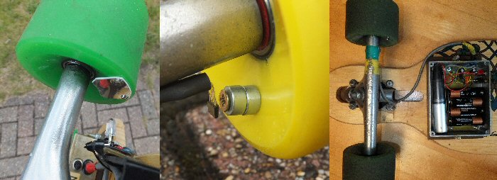
Fig. 1. From left to right: i) the IR detection technique (see ref [1] for details), ii) the magnetic sensing technique (before water proofing the Hall effect detector, see ref [2]) and iii) longboard showing the speedometer electronics underneath the board (protective lid removed). In iii) we can see the 4 AA batteries, the usb data logger (the vertical silver looking object) and some of the electronics.

Introduction
A year ago I published a paper describing a relatively simple speedometer that could be constructed and fitted to a skateboard or longboard (or even a bicycle) [1]. This used an Infrared (IR) LED and an IR TV remote control sensor to detect the rotation of one of the wheels and convert this into a voltage (proportional to speed) which is measured using a removable data logger Fig. 1i. A simple empirical calibration constant (dependant on the wheel size etc.) can then be used to convert the logged data into speed (mph, kmh^-1 or ms^-1 etc.)[1].

Since then I have developed a simpler (less component count) version that uses magnetic sensing instead of IR [2], Fig. 1ii. The two different techniques complement each other showing how the same physical phenomena can be measured in different ways. I also added a push switch on the device to provide out-on-location data markers to highlight especially interesting data or for calibration for example [2]. So far (July 2013) I have journeyed over 600 miles on the longboard and logged 100's of hours of data.

Data analysis
In the original paper I briefly mentioned that the speed data could be downloaded to a spreadsheet for analysis [1].
I also mentioned that simple numerical methods might be applied to this data to integrate and differentiate the data to derive distance and acceleration information.
Here I show how to do this in detail.

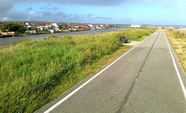
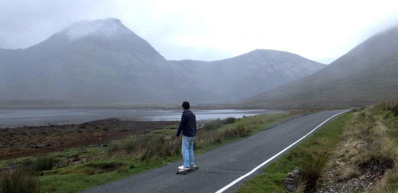
Fig. 2. Widewater near Shoreham in Sussex (UK) looking east.
This flat path is a safe place to make skateboard and longboard measurements and a great place to be able to get up a good speed on an easy route.
The sea is on the right hand side while the inland lagoons are on the left.

West of Shoreham, at Widewater, there is an ideal stretch of flat path that runs between the sea and some inland lagoons (see Fig. 2). This path is about a mile long and is almost a perfect spot to check the data logging equipment and to get up speed safely. You can easily keep-up a steady speed over this mile and so timing how long it takes provides a simple way of determining an average speed. Although this is not the most exciting high-speed or down-hill adventure, I present the results as an example of what can be done with the data rather than what can be done on a longboard or skateboard. Obviously what I describe here can be applied to more adventurous trips.

Setting up the logger and downloading
For my experiments I used a reasonably priced usb data logger by Lascar Electronics (type: EL-usb-03) which can take a maximum of about 32,510 measurements (logs) and accepts a 0-30V input. These loggers can be set to start recording using the software. The device includes its own quartz crystal clock so that the logger keeps time fairly accurately (ca. drifts a few seconds a day or less depending on the temperature changes etc.). I set-the data logger to the fastest recording rate which is one measurement per second (in this setting it can therefore log for ca. 9h hours). Once you have been out on the skateboard or longboard the logger can be removed and fitted into a PC via the usb socket to download the data, Fig. 1 iii. The logger comes with its own software which will display the data on a graph or in table form. The program also allows the data to be exported into a spreadsheet (Excel) for analysis.

As our data logger is only making a measurement once every second, rather than thousands or millions per second (e.g. as a spectrum analyser or digital oscilloscope would do) our numerical analysis will be quite low resolution. But the basics discussed here can be applied to more sophisticated logging techniques.

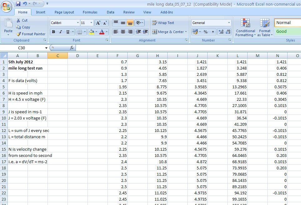
Fig. 3. Screen shot of the Excel spreadsheet containing various columns of data based on the raw voltage data logged while out on the board. Column F is the voltage data from the speedometer electronics.
H is the scaled data to mph, J is scaled to ms-1, L is the distance travelled (m), while column N is the acceleration (ms-2).
Note: see text for details of interpreting these numbers, their resolution and number of places of decimal.

Fig. 3 shows a screen shot of the Excel spreadsheet showing all the columns of data and analysed data in columns F, H, J, L and N. This data was collected for a run along Widewater in July 2012. The run was about 1 mile taking about 300 seconds (5 mins), see Fig. 3 column F. This data and the following analysis is available as a download on my web site (see end of the article [4]).

I copied the voltage data into column F. The data was copied right at the top of the F column so the first data is at the first second. You can think of this as the average speed over the first second so we don't need to worry about starting from 1 rather than 0. All other data points are therefore so many seconds from this start time, shown by the automatically generated row numbers on the very left hand side of the spread sheet.

As column F is the voltage data from the speedometer electronics, the next step is to convert this to speed e.g. miles per hour (mph) or meter per second (ms^-1) simply by multiplying by a constant of proportionality (see the original article on the speedometer [1]).
Speed = constant x voltage data

These constants are empirical ones dependant on the size of the wheel and the number of sensing elements (i.e. the number of mirrors in the IR set-up or number of magnets in the magnetic sensing circuit). The constants can be estimated in a number of ways including measuring the time it takes to run a known length to estimate an average speed or by working out the constant from this data or by using a Gym 'rolling road' type exercise machine [1].

Resolution of speedometer, spreadsheet analysis and number of decimal places
The speedometer is not a state-of-the-art device but it does give interesting average speed data for the skateboard or longboard. If only one mirror, or one magnet, is used to detect the wheel rotation then the position resolution will be of the order of the circumference of the wheel (ca. 22cm for a 70mm longboard wheel). If more mirrors of magnets are used then the resolution will be proportionally better. If the single magnet apparatus detects 10 pulses we can say, to a first approximation, that the longboard has moved 10 x 22 cm = 2.2m ± 0.22m. The circuit does not actually count pulses but measures the average voltage created by the pulses (a standard technique in electronics). For a constant pulse train (constant speed on the board) this will produce a voltage which can be measured by the logger. The averaging circuit creates a DC voltage from the pulses that is noisy (depending on the speed) and this will be one limitation on the resolution of the recorded data. The speed data derived from the speedometer should therefore understood to be approximate perhaps an of ca. 10% accuracy.

One of the problems of using an electronic calculator or a computer spreadsheet is that calculations using the low resolution speedometer data often generate numbers with far too many places of decimal. For example in the 16th second of data logged in Fig. 3 we see a calculated total distance travelled of 64.0465 meters (column L). The student should recognise that this should realistically be read as ca. 64 m and that it does not imply that we have really calculated the total distance as 64m + 4.6cm + 0.5 mm. In other words although the spreadsheet produces figures to several places of decimal we are not in any way measuring the total distance to a precision of less than a millimetre! I have not truncated the values in the columns because the students own calculations will no doubt create similar numbers but the student should be aware what these numbers realistically mean.

Producing the speed data
For my wheels and experimental set-up the mph constant was 4.50 and the ms^-1 constant 2.03. So we need to multiply all the voltage data points in column F by 4.50 to produce the mph data in column H and by 2.03 to produce the ms-1 data in column J.

For those new to spreadsheets one way to do is to click on the first entry in column H and in the '=' Formula bar or box in the menu bar of the spreadsheet click on the box and then type in "= 4.5 * F1" and press enter. This will multiply the value of the first voltage data point (0.7 volts) in the first row by 4.5 to give the corresponding mph speed for H1. H1 will therefore become 0.7 x 4.5 = 3.15 mph, see the screen print out Fig. 3.

Now click on this box (H1) and 'copy' (right click using the mouse or equivalently press the 'control' and 'c' buttons together). This will copy the function formula i.e. the '4.5 x F1' rather than the value 3.15 at n = 1. Now highlight all the rest of the column (either using the mouse or by pressing 'control' and 'a') and paste.

Alternatively, if you hover the mouse over the H1 box you will see a small black square on the bottom right hand side of the square, click on this and you can 'auto fill' the whole of the H column data (If this does not come up then you can simply drag the small black square downward to the end of the column).
The H column should now be filled with each individual voltage data of the F column multiplied by 4.5 to give the speed in mph at each second. We do the same for column J but use the 2.03 factor to produce ms^-1, see Fig. 3.

The columns can now be plotted out by highlighting a column and clicking on 'insert chart'. Once created I usually right click on these graphs and select 'move chart' and then 'new sheet' so that they are all on their own page but it's your preference here. The axis units, ticks mark units and labelling can be edited as desired.

As the row information / numbers corresponds to seconds from start of the trip we don't have to worry about scaling the horizontal axis as its already in 'seconds but it would have to be scaled by 1/60 if we wanted the scale to be in minutes for example. But if the logger had been set up for a measurement every 10 or 100 seconds then we would have to modify the time axis accordingly.

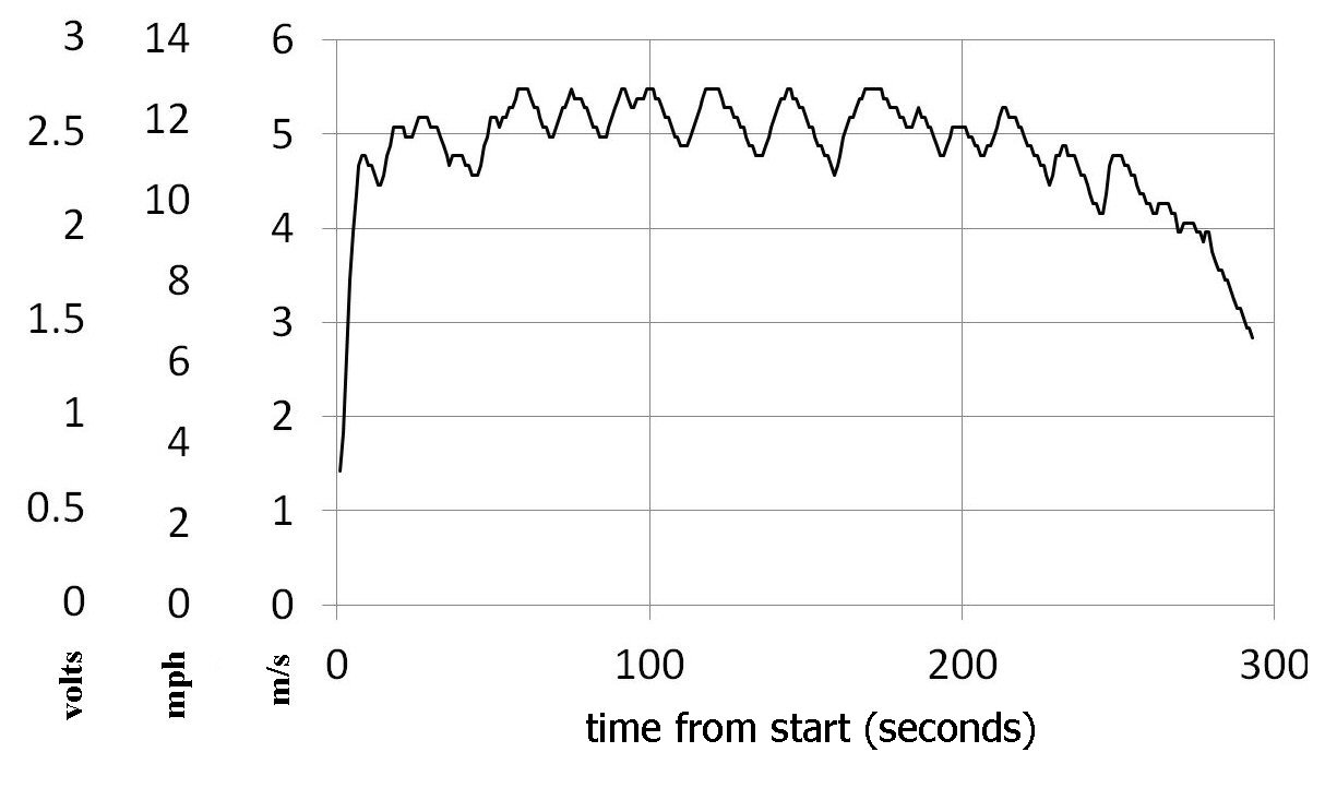
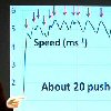
Fig. 4. Three representations of the data collected by the skateboard / longboard speedometer data logger against time from start (seconds). The vertical axis on left hand side shows i) the raw voltage from the data logger (volts), ii) the scaled values in mile per hour (mph) and iii) the speed in ms^-1 (m/s).

The speed plots show that the speed was fairly constant over the test run and we can clearly see the speed peaks each time I push the board with my foot. There are about 20 pushes over the 300 seconds (ca. 5 minutes) of the test run, showing that I needed to top up the board with a push every 15 seconds or so. You can also see that I was able to develop a steady speed during the main part of the run and by eye you can estimate it was an average speed of about 5.0 to 5.5 ms^-1 or 11 to12 mph.

MKS, mph and ms^-1
Although we might talk about a car or bike speed in mph it's good to stick to MKS units for science, so from now on we will use the ms^-1 data (in column J) for the rest of the analysis.

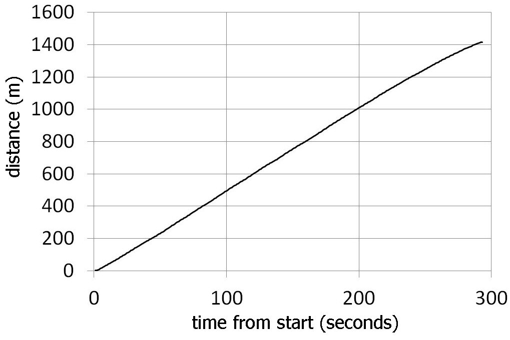
Fig. 5. Integrated speed data - a plot of the total distance travelled from the start (in seconds).
We can see the total distance travelled in the 300 seconds is about 1400m and from the gradient we can estimate the average speed (ca. 5ms^-1 or 11 mph, see text).

This process of summing the data is a crude form of numerical integration. In calculus the integration of velocity is distance.
(we assume the constant of integration is zero at the start).

If we had set the logger to take a measurement every 10 or 100 seconds (which we might do for a long trip) our distance between each measurement would have to be multiplied by these factors. Obviously the smaller time step between each data points the better resolution in the analysis.

For distance calculation we will sum up each value of 1 x J i.e. for each speed data point, as a running total and put the value of the running totals in column L.

L1 will be the total distance travelled in the 1st second:
L1 = J1 x 1 = 1.421 m

L2 will be the distance travelled in the 1st and 2nd seconds:
L2 = J1 + J2 = L1 + J2 = 1.421 + 1.827 = 3.248 m

L3 the total distance travelled from start to the third second:
L3 = J1 + J2 + J3 = L2 + J3 … and so on.

L(n) is the total distance after n seconds;
the sum of all the J values from 1 to n. So L(n) is the total distance travelled n seconds after the start.

Calculating a running total
The way to do a running total on a spreadsheet is very clearly described on the Microsoft web site [3]. We will create a running total in column L using the ms^-1 data from column J so that the results will be in meters.

Start by clicking on L1 and typing in the value of the distance in this first second (1.421 m). This is the value of the speed in ms^-1 x 1 which of course is simply the numerical value of the speed in J1.

Then click on L2 and in the '=' box type in '=J2 + L1' which will give the sum of the first two distances in L2. Now click on L3 and type in the box '=J3 + L2' and press return. L3 will now have the running total in it. Click on L3 and copy ('control' and 'c') and then highlight the rest of the L column (control and 'a') and paste. The L column will now be full of the running totals; the total distance covered at every second from the start of the skate journey.

Another way of doing this is to fill in L2 and L3 as above but when you get to the L3 stage point the mouse to the bottom right of the L3 box. Here you will find a small black square, if you click on this there is an 'auto fill' option that will fill the rest of column L with the running totals (if the autofill fails to appear, simply drag the small black square down to the end of the column).

If you look down the L column you can see that each subsequent value in L increases as time passes, as you would expect for the total distance travelled. Note: this is the total distance the wheels have travelled if you could 'straighten out' the path. So going around and around in a circle or going back and forth will still 'clock up' more and more distance (we are treating the speed as a scalar rather than as a vector velocity).

The data is plotted out in Fig 5. The first thing to notice is that the journey was quite uniform, we can immediately read off from the graph the total distance travelled (or we can go to the end of column L and read this off): in this trip we travelled 1416 m. Now one mile is 1610 m so the run on this day was just under a mile.

The gradient of the graph is the distance / time which will give us the average speed for the whole of the journey. You can see in this case that it's much easier to get this average from the integrated data than it is by trying to guess an average by eye from the varying speed plot of Fig 4. If we look at Fig. 5 we see that from 100 to 200 seconds (dt = 100 sec) into the journey the distance (s) changed from 500m to 1000m (ds = 500) so the gradient on this part of the graph m is:
m = ds/dt = v = (1000 – 500) / 100 = 500 / 100 = 5 ms^-1

Note: If the total distance travelled is known accurately (e.g. by GPS, Google maps or ordinance survey map) then you could use the results of this data to recalibrate / check the accuracy of the speed calibration constants. For example you could modify the 4.5 constant for mph and the 2.03 constant for ms^-1.

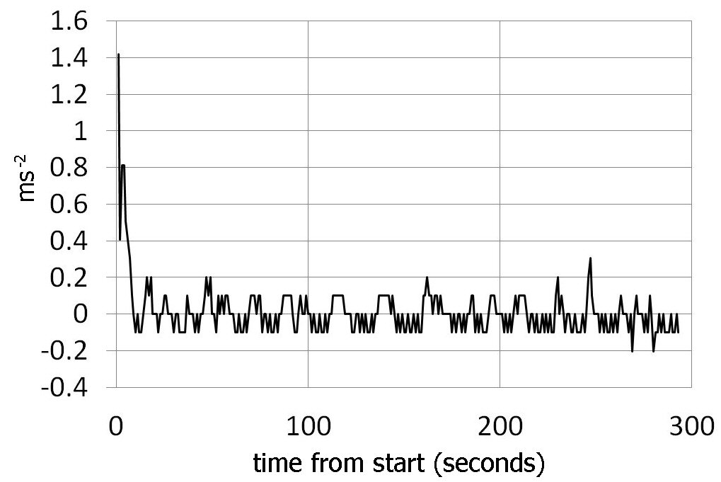
Fig. 6. The acceleration data (vertical axis ms^-2) v time from start (seconds). This was generated by calculating the rate of change of speed (ms^-1) every second from one second to the next. As the run was so smooth notable accelerations are only observed at the start, as we speed up. Decelerations are observed near the end when we start to slow down. The 'noise' / fluctuations during the main part of the trip is partly due to the speeding up and slowing down experienced during each push of the board.

The way we do this in the spreadsheet is to form another column, say N for this new data. N1 will simply be the value of the speed at J1 so we simply copy this value from J1 into N1. Then we click on N2 and press enter and in the equal box type '=J2-J1' which will give us the change in speed from the 1st second of travel to the 2nd second of the trip. Note the order: J2 first minus J1.

Fig. 3 shows that the entry for N2 will be:
N2 = J2 - J1 = 1.227 - 1.421 / 1 = + 0.406 ms^-2
Note: positive values represent acceleration, negative values represent deceleration.

Copy the highlighted entry into N2 and paste into the rest of the N column as we have done before so that the rest of the N column becomes populated with all the other acceleration values. All the N entries should now contain the accelerations during the trip. Here we are not running any total but just the difference in speed J(1) - J(t-1) over 1 second = the acceleration, at any time (t) from the start.

A positive value will represent acceleration from the previous second while a negative value will represent a deceleration. This N column data of the accelerations can be plotted out as before and is shown in Fig. 6.

As the run was so uniform we would not expect too great a change in acceleration and this is clear from the plot. We do however see a strong positive peak at the start as we pick up speed from standing and later we see negative peaks as we slow down at the end of the trip. Each push (ca. 20 pushes, see speed plots above) creates an acceleration and afterwards a deceleration as the board slows down but these are relatively small values and so contribute to a 'noise' level, or fluctuations, for the main bulk of the journey on the acceleration plots. In principle if we multiply the acceleration data by the mass of the person (plus the longboard mass) we should get the forces he or she experience (from Newtons F = ma). However as the skater may be moving around on the board, going around corners and varying his or her height etc., this simple analysis may not give very reliable values for the real forces in practice.

Dealing with markers
In later versions of the speedometer I added a button so that the recorded data could be 'marked' while out on the road. I did this because if you are recording a maximum of say 9 hours of data it's not always easy later on (when downloaded) to recognise what part of the data corresponds to what part of the trip.

I therefore included a marker press switch that you simply press to highlight a particular part of the data. When the switch is pressed it wires the data logger to the speedometer electronics positive supply (e.g. 6V) which produces a strong signal on the data never normally seen in the speed data. This marker signal continues as long as the button is pressed (you need to hold it down at least as long as the data logger measurement period).

You can press the button just before an interesting part of the journey comes up and then immediately after to 'mark' this part of the data. When downloaded this special part of the trip will show up sandwiched between the two high peaks ('markers') generated by the marker push switch.

Although the markers help to divide the data up nicely, we may not want this marker data to be incorporated into the speed, distance or acceleration calculations. In the analysis described in this paper I deliberately only copied the data between the set of markers (leaving them out). On a longer journey, perhaps with more than one set of markers, you can simply replace the marker signals by typical values found adjacent to the markers.

Sample spreadsheets
If a teacher or pupil wants to go through the analysis but does not want to undertake the project of making the speedometer I have included examples of voltage data from three trips on my web site [4]. These spreadsheets can be downloaded and used as representative data for class or homework analysis for example. I have also included the complete July 5th 2012 mile-long spreadsheet of the Widewater data containing the F to N column data described in this article including the graphs.

Summary
Although this analysis is very simple it allows us to explore the data generated by the skateboard speedometer and so develop what can be done with the measurements. It's a simple way to start exploring numerical methods before more advance techniques are considered (e.g. Trapezium rule, Simpson's rules etc.).

References
[1] Skateboard / longboard speedometer project. J P Hare, Phys. Educ. 47 (2012) 409-417.

[2] Longboard Speedometer
CSC Skate page

[3] microsoft excel help

[4] example data and spread sheets can be found at my CSC web site:
spreadsheet

Sussex University science series

Longboard Part 1 Speedometer	Longboard Part 2 Physics	Longboard Part 3 Chemistry	Longboard Part 4 Numerical Analysis	More soon

---

THE CREATIVE SCIENCE CENTRE

---

Dr Jonathan Hare University of Sussex, Brighton.
e-mail: j.p.hare@sussex.ac.uk

home | diary | whats on | CSC summary | latest news

---