Skateboard / longboard speedometer project
Dr Jonathan Hare, The Creative Science Centre, University of Sussex

Return to CSC skate page

This article has been published and is reproduced here by permission. J P Hare, Physics. Education, 47 (2012) 409-417.
for a free download from the IOP web site go to: Longboard Speedometer

There were a few typos and referencing mistakes in the original article (some confusion over foot notes and references) so this web version has been corrected.

NEW ** click here for latest up-dates, modifications and alternative techniques ** NEW

Please also see the MKI, MK2 and MK3 versions

Abstract
A simple low cost Infrared LED speedometer is described that can be fitted to a skateboard, longboard or even a bicycle to measure speed. Notes on building, setting-up and calibration are given. When used with a low cost data logger continuous measurements of speed can be made while out-and-about. The device forms an interesting science club project and would be a great introduction to potential physicists and engineers to scientific instrument design, testing and calibration as well as to generate lots of their own interesting data to analyse.


MK3 MK3

Fig. 1. Longboard skateboard with IR speedometer circuit attached underneath the board. The electronics is housed in the small di-cast box under the board (right).


Introduction
Skateboarding has been around for at least 60 years but in its popular form since the seventies [1]. Recently longboarding has started to become popular with adults as well as with children [1]. The longboard has larger wheels and wider trucks than skateboards making it more stable for adults as well as better equipped for commuting and long trips. YouTube videos show that people are now using longboards on 2000 km treks! [2]. As longboards are generally better made and larger than skateboard they are easier structures on which to develop instrumentation and measurement equipment. It's great fun to combine science, instrumentation and longboarding.


MK3

Fig. 2. Schematic of the IR speedometer showing the IR transmitter, IR detector (receiver), the pulse shaper and average or integrator circuits.


How it works
Here we use Infrared (IR) light to monitor the speed of rotation of one of the wheels. Light from an IR LED is directed at one of the wheels. The wheel has a small reflector fixed to it (see below) and when it rotates into position it reflects a signal back to an IR receiver. On reception of the IR beam the receiver o/p pulses low (0V) for a short period. These pulses are too variable to monitor directly but we use them to trigger a timer (555 No. 2) which produces pulses of regular duration (ca. 15 ms, see below). These positive going pulses are then averaged using a simple low pass filter / integrator circuit (Ri and Ci) which smoothes the pulses creating a DC voltage proportional to speed. Data Logging allows measurements to be made out-and-about. A simple constant calibration (K) allows the voltage data to be converted into mph or kph etc.

The transmitter circuit consists of an astable oscillator (555 No. 1) which pulses (modulates) the IR LED at 38 kHz. We use a standard IR LED as used in remote control systems (e.g. TV, cd, cable etc.). A cheap commercially available IR detector (as used in TV remote control systems) is used (Note: we are using this device out-of-spec but its use greatly reduces the components needed). These are sensitive to IR modulated at 38 kHz (hence the Tx frequency). Although these devices are very cheap they have built-in filters and tuned pre-amps to give good stability and sensitivity. We make use of this reliable remote control spin-off technology which provides much better noise immunity than a visible light beam circuit.


Component Listing
Resistors
1 x 100R, 680R, 4k7, 68k, 100k
2 x 10k
1 x 20k 10 turn mini-potentiometer

Capacitors
1 x 0.01uF, 0.22uF
4 x 0.1uF
2 x 1nF
3 x 100uF 16V

Semiconductors
2 x NE555 timer chips (dont use the CMOS versions as they may not supply enough current to power the IR LED)
1 x IR remote control detector (TSOP4838 e.g. Rapid Electronics S/N: 55-0905)
1 x IR LED (Rapid Electronics S/N: 58-0112)
2 x 1N4148 silicon diodes

Misc.
1 x metal box (120 x 95 x 34 mm, e.g. Maplins N90BQ)
1 x ON/OFF switch
cable grommet
20 cm of 3 way cable for sensor
data logger (to fit box)
I also gave the metal box a couple coats of varnish to protect from the weather.


The electronics
The circuit involves a straight forward use of the ubiquitous 555 timer. I used two separate 555 for my prototypes, to help in fault finding, but a double 556 timer could be used for compactness. All the components are cheap and easy to obtain. None of the components are very critical but good quality components should be used for the timing capacitors (e.g. use metallised polyester for the 1nF and 0.22uF capacitors). The total cost of the electronic components should be about 10 pounds / Euros. You might even be able to take an old cd or TV and controller apart to use both the IR transmitter LED and detector IC etc.

Note: A specialised frequency-to-voltage (e.g. LM331) or techometer (e.g. LM2917) IC could have been used instead of the second 555 timer. This would probably produce a more linear and wider ranging circuit but in this design I have chosen to use the humble 555 because it is very cheap and well know to GCSE and A-level electronics / physics students and teachers. Other designs, modifications and up-dates will be explored on my web site [5].
** click here for latest up-dates, modifications and alternative techniques **

The integrator circuit used to average the pulses from the second timer comprises Ri and Ci. With the values given (10k and 100uF) we get a time constant of about τ = aprox. Ri x Ci = 10,000 x 0.0001 = 1 second. I found this was a good compromise between reducing the noise generated by the pulses while still responding well to quick changes in board speed. Ri and Ci can be adjusted for different averaging response times. The integrator is fed from the second timer via a diode, so it has a fast response time (τ) but slower decay.


MK3

Fig. 4. The IR detector (black square, to the left of the truck) and IR transmitter LED (clear / white, to the right of the truck) fitted to their own small piece of circuit board. The two devices point toward the side of the wheel. The detector receives an IR reflection from the mirror (not visible in this photo) attached to the back of the wheel.


I used a separate circuit board to hold both the IR transmitter LED and IR receiver near to the wheel. Both these devices point toward the back of the wheel. When the mirror reflector comes into position the IR is reflected back onto the receiver, see Fig. 4. Once the circuit has been tested it would be worth enclosing the IR LED and detector it in a small box to provide protection from being knocked (some clear plastic boxes are transparent to IR which would limit the number of holes required and provide some extra weather proofing).


Alternative sensing technique - magnetic detection
click here for latest up-dates, modifications and alternative techniques


Setting-up
Arrange the IR LED and IR detector module a few cm apart so that they are pointing at each other. Adjust the IR transmitter frequency using the 20k (ideally multi-turn) potentiometer. Start with the full 20k in circuit and then reduce the resistance till the frequency is ca. 38 kHz. Use a scope or frequency counter attached between ground and pin 3 of the first 555 timer. With no modulated IR signal present the IR detector o/p is high. Test point 1 (T/P 1, see circuit) will be ca. 5V. When the 38 kHz modulated IR LED is correctly aliened (pointing at the detector a few cm apart) T/P 1 will go low (0V). I found that some IR LEDs do not create enough IR light to permanently keep T/P 1 low. If the LED produces a pulse but not a constant 0V signal this unfortunately is the case. If you have this problem lower the value of the series resistor (e.g. reduce from 680R to say 330R). It's worth trying out a few different types of IR LED to see which performs the best. I found that the IR LEDs seemed to vary in performance. I have used a 'High Power' version [3].

When you get this to work, check the electronics is functioning properly by waving a finger or ruler (or other solid object) between the IR LED and the detector. The voltage on T/P 1 will pulse as you do this, triggering the second 555 timer. The faster you do this the more pulses will be generated and so the higher the voltage will rise on the averaged o/p (measured on a meter or the logger).

With the electronics set-up on the longboard (or skateboard), rotate the wheel so that mirror will reflect the IR LED beam onto the IR detector. You should be able to get T/P1 to go low, and stay low. When you spin the wheel T/P 1 will pulse, triggering the second 555 and producing an o/p proportional to wheel speed.

Important Note: If you readily get T/P 1 pulses when you rotate the mirror / wheel it may not necessarily mean all ok. You need to be able to reliably get T/P1 to go permanently low (0V) when the mirror is in position (when still). If you cannot get this preliminary result, the speedometer o/p voltage will be erratic and you won't record reliable speed measurements (even though it appears to be responding ok). To make sure you can get the correct T/P 1 signals, experiment with the LED / detector alignment, reduce the gap between the LED / detector and mirror, try a better IR LED or reduce the LED series resistor (e.g. from 680R to 330R, 220R or even 100R).


MK3

Fig. 5. Speedometer fixed underneath a standard skateboard. This version uses four mirrors attached to a wheel, as the IR reflectors (see reflector photos, Fig. 6 for details). The small data logger can be seen in the left hand. You can also see meter sockets which are useful for making checks on the o/p before going out on a trip.


The circuit will operate from 4 - 6V so 3 x AA 1.5V batteries are ideal. Lithium batteries provide long life and are light weight. I made my own printed circuit boards (pcbs) for the prototypes but strip board or perf-board could be used instead. In later versions l covered the electronics using a glue-gun to reduce moisture problems. I used a di-cast metal box for strength, a water proof cover for the ON-OFF toggle switch and also tapped the edge of the lid to try and reduce water getting in. It's also useful to have the o/p signal wired to a small socket on the side of the electronics case. This way you can do a last minute check by spinning the wheel with your hand and monitoring the o/p with a meter.


MK3

Fig. 6. Various methods used to reflect the IR beam from the wheel: 4 mirrors, white paint spots, a hemispherical pin head and a small piece of plastic mirror attached to the wheel (with two nails). This last method has proved most effective (see text).


Reflector - measuring rotation
The IR beam from the LED reflects off the mirror attached to the wheel back onto the detector. My first attempt at getting this to work used four plastic mirrors glued to a makeshift tin sheet holder screwed into the back of one of the wheels (see skateboard results below). This worked very well but it was a bit fragile. I then simply tried painting a white spot on the side of the wheel using correction fluid (Tipex) or white paint. Amazingly this reflected the IR very well but the flexing of the wheels resulted in the paint crumbling or peeling off in just a few hours.

Despite the longevity issues, correction fluid can still be a quick and convenient way of testing the equipment in the early stages of the project. I then tried a long pin with a hemispherical head which I hoped would reflect back the IR over a wide range of angles as the trucks moved around. This worked but unfortunately I did find there was some signal dropped-out, particularly on tight bends etc.


My current set-up uses a small piece of plastic mirror ca. 1 x 1.5cm fitted onto the side of a wheel using two 1.5cm long (large head) brass nails. Note: I used a G clamp to force the nails into the side of the wheel - it's no use trying to hammer them in to polyurethane! I was worried the nails might split the wheel, but no deterioration has been observed over several months, in all sorts of conditions both in the summer here in the UK and on a trip 'down under' in New Zealand (their winter).


15 ms pulses, revs per sec and maximum speed
Why set the second 555 timer for 15 ms pulses? With this pulse length we have a maximum number of 1000 / 15 = 67 pulses per second. If we are using one reflector on the wheel we will get one pulse per revolution. This will correspond to maximum detectable speed of 67 revolutions per second. For my Longboard wheels with a diameter of 76mm the circumference is ca. 0.24m and so 67 of these correspond to about 16m / second which is about 58 km / hour or 36 mph. This is a good maximum speed but it also means that lower (more realistic) speeds still produce a decent output that can be measured.


If you want to measure fast speed then you really only need one mirror. However if you still want good resolution at low speeds it will be worth using more mirrors but then reducing the second 555 pulse length by reducing Ct. I have done this for the skateboard version (see example 1 in the results section below) where I used ca. 3ms pulses instead of 15ms. By reducing the pulse length you get larger maximum speeds recordable and by increasing the number of mirrors you also get good resolution at the lower speeds, but at the price of more complexity (more to go wrong).


Maximum and minimum speeds
The integrator circuit (low pass filter) averages the positive going pulses from the second 555 timer creating a voltage proportional to the number of pulses per sec (i.e. board speed). As discussed above this occurs till the pulses are so numerous that the 555 is ON almost all of the time which represents the limit, or maximum speed recordable. At very low speeds the individual low frequency pulses will tend to produce a small step change in o/p rather than a gradual change in o/p and so low speeds will appear noisy and slightly larger than they should be. Both very low and very high speeds will therefore tend to create non linear responses on the o/p of this circuit (see the 'treadmill' results below). For most use out-and-about this will not represent much of a problem.


Logging data
Small stand-alone data loggers are now available cheaply [4]. They can be set-up to make regular measurements over many hours. The data can be easily downloaded (via usb) to a computer and analysed / modified on a spreadsheet. I set up my data logger to take one reading every second. For my logger this means I can continuously log for about 7 hours. When downloaded, the data consists of the date and time tabulated next to the voltage. 1 log every 10 seconds is also possible if you wanted to log on a longer trip. However longer gaps between measurements make it difficult to reliably measure the relatively quick changes in speed of a skateboard. However this logging rate might be fine for using on a bicycle for example.


Modern data loggers seem to have an input resistance of 100k or greater so they do not load the integrator to any great extent. If a lower resistance measuring circuit is going to be used then an op-amp voltage follower (unity gain amp high input impedance circuit) should be used after the integrator.

My data logger can accept a 0-30V i/p via two wires that screw into the logger i/p / usb socket [4]. I used a large elastic band (or bungee) to secure the connector to the logger so that it did not come loose with the vibrations while skating around (see Fig. 5).


Calibration
Obviously one way to calibrate the speedometer is to note the time it takes to skate at a relatively constant speed over a known distance (speed S = distance / time). I found Google earth useful for working out distance but of course an ordinance survey map would be good too. You can then plot out the logged voltage and, by eye, draw a line through the average voltage V. For a more accurate calibration you can sum all the measurements collected by the logger and divide the total by the number of measurements to obtain a better estimate for the average V (see results section below).


The calibration constant K, to convert the voltage into speed, is then found by dividing the average speed by the average voltage V i.e. K = S / V. Of course you will get different values of the calibration constant K if you convert to m/s, km/h or mph etc.

Note: this calibration constant is dependent on the second 555 pulse length, wheel size, number of mirrors etc. but once determined you don't need to do it again so it will be the same for all trips and tricks while out on the board.


MK3

Fig. 7. o/p from the longboard speedometer at various speeds on the treadmill. The low frequency pulses created at low speeds tend to be produce slightly larger (and more noisy) outputs than expected making the graph slightly non-linear. Hence the 0-2 mph data is a little larger than expected (although the accuracy of treadmill machine was unknown). Also at very high speeds the o/p will limit to about the supply voltage (see 'maximum' and 'minimum speeds' sections above).


Testing on a treadmill
I tried towing the skateboard / longboard behind a car at various speeds on a quite spot in the country. This is not only dangerous but without a human weight on the board every bump and crevice on the road surface leads to all sorts of spurious results. To overcome this problem Varndean College (Brighton) very kindly let me use their gym treadmill (rolling road). We set-up the treadmill for a particular speed and placed the four wheels of the longboard down onto the moving surface to see how the skateboard speedometer responded. I used a data logger and also wired a DVM on to the output to record results. The treadmill speeds were set for 2, 4, 6, 8, 10 mph (the safety cut-out was ca. 11 mph so I could not go higher).

For zero speed, no pulses will be produced by the circuit and so the o/p will be zero. For low speeds a low rate of pulses results. At high speeds the pulse train is averaged by the low pass filter producing a nicely increasing voltage, but being a low pass filter the low frequencies pass through quite easily creating slightly larger signals than we would like. The recorded voltages for low speeds are therefore slightly higher (and noisier) than might be expected and so the graph is slightly non-linear at low speeds. Note: the non-linear response of the low speed rolling-road tests shown on the graph may also be due to the inaccuracies of the machine which were unknown. Once above ca. 2 mph the o/p is far more steady for any particular speed (the DVM was stable to a few percent). If we ignore very low speeds (< 2 - 3 mph) you can see from the data (Fig. 7) that the response is fairly linear.

The reciprocal of the gradient (1/m) allows us to estimate the calibration constant K. For the treadmill results this gives a value of about K=5 mph/volt (Note though that the accuracy of the treadmill speedometer was unknown). This is close to that determined by the 'out on the road' tests for the longboard (see example 2 below) which gave K = 4.5 mph/volt. Overall you can see that the o/p is basically proportional to speed above ca. 2-3 mph.


Data analysis: speed, distance and acceleration
The logged data can be loaded to a spreadsheet for analysis. The voltage data can be multiplied by the calibration constant K to give the speed (see examples below). If we set-up the logger to take one measurement per second then each data point is also equal to the distance travelled in 1 sec (distance = speed x time = speed x 1 = 'speed'). So if we sum all the 1 second calibrated data then it will give us an estimate of the total distance travelled. Obviously this value will depend on the accuracy of the calibration constant. We could also sum as we go through time to get the total distance travelled at any time and plot this out to give a distance time graph. This is a crude form of numerical integration with respect to time. If we look to see how the speed changes from each second to another we can also get a crude idea of the rate of change of speed and therefore the acceleration. This is a crude form of numerical differentiation with respect to time. Spreadsheet programmes like Excel have all sorts of data analysis tools that can be used to investigate the data.


Results - out and about
Please read again the notes on setting-up so that you can be sure that the IR LED is producing a strong enough signal for the IR detector to lock-in-to (i.e. make sure TP 1 voltage is zero when the mirror is aligned still). Once this is done everything should be working so you can calibrate the speedometer o/p and start making measurements skating out-and-about.


Example 1: skateboard (four mirror reflectors)
The skateboard speedometer was my first prototype and I wasn't sure how responsive the system would be so I used four mirrors as a starting point. Each turn of the wheel will therefore produce four pulses. I used a small value for the timing capacitor Ct on the second 555 timer (0.047uF instead of 0.22uF as in the longboard see below). This produced short 3 ms pulses. The greater number of shorter pulses per wheel revolution used in the skateboard results in a similar overall response (ignoring wheel size differences etc) to the longer single pulses per wheel revolution, used in the longboard (see below).


MK3

Fig. 8. Promenade run along the coast from Lancing to Worthing (West Sussex, UK) pier. The logged voltage has been converted to mph simply by multiplying all the logged voltage measurements by the calibration constant K, in this case K = 5.37 (see text). You can see various speed changes along the route due to crossing paths [2], effect of each push to gain speed [3], deceleration with no pushing [4-5] as well as other interesting observations. Note time runs right to left to match the direction of travel on the map above.


Here you can see the skateboard speedometer tests on a sea front promenade run between Lancing and Worthing in West Sussex, Fig. 8. It was helpful to leave a blank period both at the start and the end of each calibration run (i.e. no movement) so that logged data clearly shows the active and inactive periods. From the logged data you see that it took 1038 seconds (0.28 hour) to cover the 2 mile (3.2 km). The average speed was therefore 2 / 0.28 = 7.1 mph. As the logged data varies quite a bit it is not so easy to estimate the average by looking at the plotted data by eye. So in this case I loaded the data into a spread sheet and summed all the 1 second data points (1 log / sec) and then divided this total by the number of logs (1038). This gave an average logged voltage over the trip of 1.33 volts.


The calibration constant for this particular skateboard set-up was therefore
K = 7.1 /1.33 = 5.37 mph / volt.

Peak voltages of just over 2 volts were recorded which correspond to a peak speed of about 11 mph. I have reversed the time scale to so you can see the speed progress under the map of the route. There were paths crossing the promenade consisting of ribbed paving slabs, often with people walking back and forth so I had to slow down and often had to stop for them. You can see these events marked as [2] (Note: a 'marker' not a reference) on the data.


acceleration
deceleration

Fig. 9. Speed-time (mph v seconds from start) plots showing a fairly regular period of skating (top) showing the effect of each push skating along and (below) a period of deceleration simply by letting the board slow down on the path. (Note: time runs left to right, as normal).


Between 400 and 900 seconds you can see that I was able to develop quite a good speed and slowly accelerate [3]. You can also see how the speed increases during individual pushes of the board as I skated along [3]. Towards the end of the run (900 seconds) I came into Worthing and allowed the board to come to a rest, I look around for a few seconds and then continued on to the pier [4] and you can see the variations of speed. Some of these observations are shown in more detail in Fig. 9.

(Note: In these detailed plots I have shown time developing in the normal way from left to right).


Example 2: Longboard (single mirror reflector)
I decided to use just one mirror reflector for the longboard for simplicity and durability. The following example shows it being used on a short run around a park (The Level, in Brighton). Obviously you could easily extend this analysis to more challenging trips. On the left hand side of Fig. 10 I have drawn the route on the map while on the right you can see the speed plots (logged voltage x calibration constant K, see below). I used Google maps to measure each leg of the journey so we get the total length L = 0.18 + 0.11 + 0.1 + 0.12 + 0.11 + 0.06 = 0.68 miles. The logged data shows it took 324 seconds to run around the park. This gives an average speed of

Speed = 0.68 x 3600 / 324 = 7.6 mph.


This time I simply drew a line through the plotted voltage data to estimate an average. From the data the average voltage was about 1.7 V. The mph scaling factor K for my longboard set-up was given roughly by:

K = 7.6 / 1.7 = 4.5 mph / volt
Longboard speed S (mph) = 4.5 x V (logged voltage)


MK3

Fig. 10. Looking down on The Level (Brighton, UK) showing a test-run with the corresponding speed plot (mph) against time (seconds from start).
You can see the various speed changes while out-and-about with the corresponding places on the map.


When the data has been loaded on a spreadsheet it's an easy matter to multiply all the data by a calibration constant K to get the speed in mph. From the picture of the park you can clearly see the start point (a) and the main turning points (marked b, c, d, … f). These points are reflected in the varying speed profiles on the calibrated logged data seen on the right hand side of the figure. You can also see from the data that to get from a to b for example there are about 15 peaks corresponding to 15 or so pushes while skating along the part of the run.

Obviously this is just a simple example of the sort of thing you can do with the longboard speedometer and analysis of the data on longer trips will reveal all sorts of interesting things. For example the road surface and direction of prevailing wind produce a great difference in the rate of deceleration after each push, and just a slight change in road gradient can effect the top speed and acceleration possible.


MK3

Fig. 11. 'On the road' near Wanaka, New Zealand


Final comments
In July 2011 I was invited to give talks and workshops at the ChemEd conference in New Zealand. To thoroughly road-test the device I decided to take my speed-logging longboard 'down under' into a West Coast South Island winter. The electronics worked well but I made a few modifications as a result of this quite harsh testing.

I soldered the data logger battery into the logger instead of using the internal push-fit battery holder. I filled the unused space between the electronics and lid with a piece of foam so that the electronics batteries and logger were held firmly in place even during the considerable vibration one can get on rough chip-seal roads. I found some of my data loggers become intermittent over prolonged use and in particular I had problems downloading the data to the PC. The problem seemed to be due to the poor quality generic usb connector that is used extensively in so much computer equipment. If the logger usb plug is 'wiggled' a bit, when plugged in to the PC, it usually resolves the problem. Finally the vibrations experienced while skating over a wide range of surfaces tends to loosen all screws, so do check the top lid screws regularly (and keep some spares handy).

It is hoped that this article will stimulate scientists and engineers to create their own board projects and enjoy analysing their own data measured while skating along (commuting) or doing tricks.


References
[1] The Concrete Wave: the history of skateboarding, Michael Brooke.
Warwick Pub., 2005. ISBN 1 894020 54 5 also see the 'skateboard' entry on Wikipedia for a good general introduction.
[2] Adam Colton, Paul Kent and Aaron Enevoldsen, treked in Peru-Bolivia and Morocco. Each 2000 km skate trip was on longboards. See 'long treks on longboards' on YouTube.
[3] I used Rapid Electronics components for both the IR LED (58-0112) and detector (55-0905).
[4] I used a small, very reasonably priced data logger by Lascar Electronics (EL-USB-3) that is ideal for these sorts of investigations.
The Testo 175-S2 data logger (0-10V input) is more professional (better construction and waterproof) but consequently more expensive.


Up-dates, modifications and alternative techniques


magnetic detection technique

Here is an alternative wheel rotation detection system that uses a Hall effect magnetic switch and rotating magnet instead of IR emitter, detector and mirror.

Possible problems with the IR set-up
The IR detection system relies part on the out-of-spec. properties of the IR detector. The part I used is now no longer being produced but it is still currently available from suppliers. Eventually though it may be hard to obtain and I cant vouch for the effectiveness of other (similar or replacement) devices. Further to this the IR transmitter is fixed to the board while the reflecting mirror is fitted to the wheel that may well be steering about a bit. I therefore wanted an alternative method that would not be effected by wheel and truck movement. Its also fun to try another detection technique and get similar data in a different way.

magnetic detection IR detection

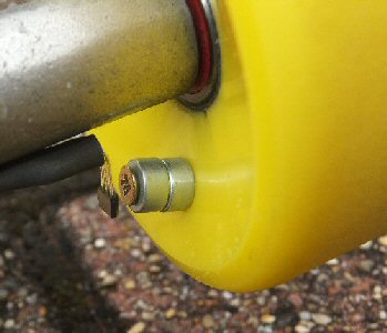
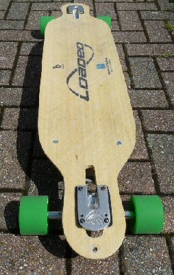
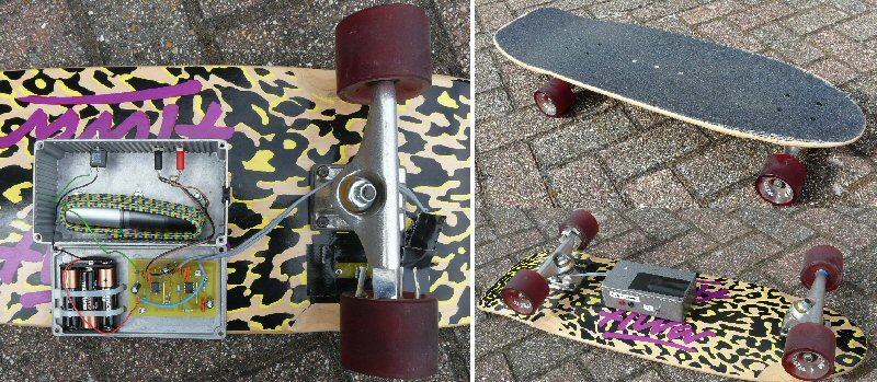
Left: the Hall effect magnetic sensing system. The magnet is fixed to the wheels and rotates into position once every rotation. The magnetic field sensor (small black device) is mounted on the truck so that it is close to the rotating magnet as it passes by. Right: the original IR detection system. As we have discussed above; IR light from an IR LED reflects off a mirror that is in position once every rotation. The reflected light falls onto an IR detector. Each technique produces pulses that can be signal processed and averaged to produce a voltage proportional to speed.

Here we use a magnet attached to the wheel instead of a mirror. As the magnet rotates it triggers a magnetic Hall Effect switch (A3144) to provide the rotational speed pulses. The circuit uses a cheap and effective solid state Hall effect magnetic switch (although a delicate glass read switch might work for low speeds). This replaces the circuitry associated with the first 555 timer and the IR detector chip. The pulses from this device go into the second 555 in an identical way to the IR set up. So this technique has a lower component count and takes less power that the original IR system.

An advantage of the magnetic system is that the magnetic switch / detector can be fitted to the truck cross bar near to the side of one of the wheels and thus all the detector apparatus follows the movement of the wheel exactly; whatever manoeuvre takes place.

magnetic field detection

Circuit of the magnetic detection system. The signal from the Hall effect magnetic switch replaces the IR detector and from then on the circuit is the same as the IR circuit. I have incorporated a 'marker' switch that can be used to create 6V pulses. This is useful when out-and-about to highlight special interest parts of the trip, these pulses are helpful to identify this data later on once the data has been downloaded.


Magnetic detection component Listing
Resistors
1 x 10k, 68k, 100k
2 x 4k7

Capacitors
1 x 0.01uF, 0.22uF
3 x 0.1uF
2 x 1nF
1 x 100uF 16V

Semiconductors
1 x NE555 timer chips
1 x Hall Effect switch type A3144 (e-bay etc)
2 x 1N4148 silicon diodes

Misc.
1 x metal box (120 x 95 x 34 mm, e.g. Maplins N90BQ)
1 x ON/OFF switch
1 x push switch or sprung toggle switch for 'marker' pulse
1 or 2 small rare earth magnets (with central hole)
1 x small self tap screw
cable grommet
20 cm of 3 way cable for sensor
data logger (to fit box)
I also gave the metal box a couple coats of varnish to protect from the weather.

Other modifications and additions
In this version of the speedometer I have also included a push toggle switch that supplies a 6V marker signal (full battery voltage) to the logger. In the IR version I suggested leaving 'zero' signals (e.g. by delibrately not moving for a while) to try and highlight or 'isolate' periods of activity so that they can easily be tracked down later on when the data is analysed. However it was still quite difficult to unambiguisly identify spacific data as you can get quite a few 'zero' signals on a trip and its just not practical to keep stoping and noteing down the time of some particular part of the route or trick. The 'marker' switch produces 6V signals which stand out very clearly when you analyse the data.

For example, lets say the logger has been set-up to record 9 hours of data and you have been out and about recording a lot. You now want to highlight one stretch of a run for particular analysis / investigation later - how do you make sure you can locate this with so much recorded data?

What you do is press the 'marker' button for a few secnds at the start, and at the end of the special run to 'top and tail' the data. These 'marker' signals are much larger voltages than normally recorded so are much more obvious on the data than say a simple 'zero' signal (which actually might occur quite often as you start and stop on the board). Once the data has been downloaded you will clearly be able to see this 'special' data incorporated within these peaks (e.g. see '1 mile data' below).

IR detection

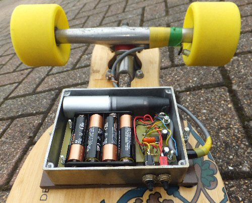
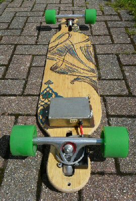
Photo under the longboard showing the electronics before the protective cover has been fitted. You can see the four AA batteries and the circuit board. The right hand switch is ON / OFF while the left is a sprung toggle that can be pressed to produce the'marker' signal useful to 'label' data during recording. The long cylindrical device is the data logger.

Apparatus description
All the electronics fits very neatly into a small dicast box. As I had a bit more room due to the smaller component count I decided to use 4 AA batteries for power longevity. AA lithium batteries would provide power for even longer and are lighter. I used the same type and size of box for the electronics as I used in the IR system as I found this worked really well over the last year in all sorts of conditions. I glued a piece of 1cm thick foam to the inside of the lid to keep the batteries in place while we rattle and roll along. I also put a tight elastic band around the logger so that the logger connector was held tight. The ON/OFF switch can be seen on the right, while the left hand switch is the marker switch. This looks like a normal toggle switch but is in fact a sprung toggle (it switches back when released) that has to be held down to create a marker on the logged data. I found it was possible to operate this switch with one hand by bending down while skating along.

The Hall effect magnetic detectors come in various forms and part numbers with a range of sensitivities. I found the A3144 device very cheaply on e-bay but others will no doubt work with some experimentation (e.g. 3141, 3142, 3134, 3213). Note: my detector only triggers with the correct face (field strength direction) of the magnet passing by. (The 3213 will respond to either a N or S pole). 
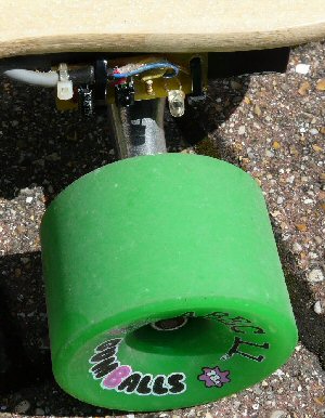
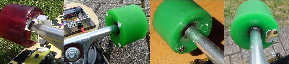
At the top of this section is a close-up of the Hall effect device (small black square) near to the magnet(s) fixed to the wheel. Also shown is the original IR set-up for comparison. This picture was taken before I covered the device in water proofing gel and shrink wrap (see below). The hall effect device and wiring was held to the truck with tape. I will up-date this page if I find a better way of attaching this (tape works pretty well even if it does not look very professional).

I used two small rare earth magnets (ca. 8mm diameter x 4 mm long each with a central hole) which I simply screwed into the side of the wheel (drill with a 1.5 - 2mm bit first) using a small self tapping screw. Note: screwing into the wheel may seem rather extreme but in practice Polyurethane is tough enough (see notes about attaching the mirror to the wheel above).


IR detection

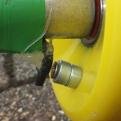
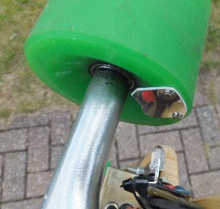
Photo showing the hall effect device covered in a protective shrink-wrap. I also used a glue gun to produce a plastic 'corner' to strengthen the bent wires of the device so that it would stay in position. Note: this photo was taken when the board was up-side-down so that the actual position of the detector in normal use is above the truck, well away from the road surface and so less likely to be knocked.

Results
To highlight what the equipment can do I have recoded some data on a relatively straight forward run along a coastal prominade path. Of course the equipment could be used on much more challenging routes. The data was downloaded from the logger when I got back home. I happened to use Orangatang Durian wheels in these tests. They are about same size as the Gumballs which I used in the IR tests so the scale factor should be the same - this is supported by the results (see '1 mile data' below). The data was exported to EXCEL and then each data point was simply multiplied by K = 4.5 to get it into mph (see calibration details in the main IR article above). The mph v time (seconds from start) data is for a run along the coast from Goring-by-sea to Shoreham (West Sussex, UK) which was about 7 to 8 miles.

The first thing I noticed was how close the magnetic sensing data was to the IR data results which was gratifying. On this design I included marker signals when the second button was pressed and these really do help identifying where the data corresponds to in terms of location. The part from 100 to 600 seconds into the trip shows the speed and progress negotiating the roads from Sea lane Goring to the start of the prominade run along the coast. There is a lot of pavement and road crossing going on so its difficult to get up a decent speed.

From 600 to 650 the signal almost goes to zero. This was where I had to stop and pick up the board to cross the main road onto the prominade. The signal did not go to zero, even though I was not skating because the wheels were spinning freely in their bearings while the board was being carried.

From 650 to 1600 seconds I race along the coastal path into Worthing, past the pier. The path now follows the coastal road and is not so wide and pleasent a route. The path continues to the Brooklands junction where I stop and use the 'marker' switch.

From 1600 to about 2000 seconds I follow the pavement around onto the sea front green at Lancing. The route is a corregated concrete path which is harder going than the tarmac paths so far skated. As a result the speed profile is more varied here.

From 2000 seconds the path goes past the lagoons west of Shoreham which I have descibed in detail below. The eight miles of the route took about 40 to 45 mins which means I was travelling at about 10 mph so the data looks about right.

Goring to Shoreham run magnetic detection

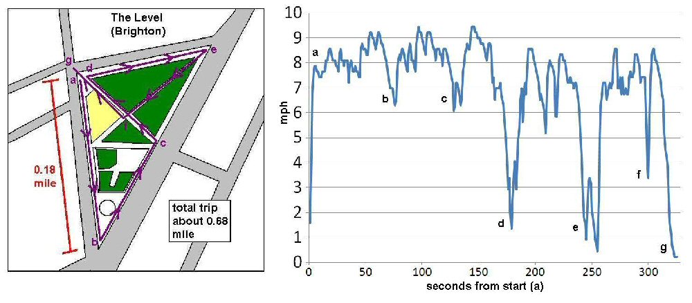
Speed data (mph) v time (seconds from start) from Goring-by-sea to Shoreham about 7 to 8 miles. The run from Goring to the junction at Brooklands (East of Worthing) is to the left of the first marker signal (large off-scale signal lines). The data between the last two marker signals is the 1 mile run along a smooth long track (see text below). Note: If you get off and carry the board you sometimes dont get zero signals. This is because the wheels often keep spinning for a while. see text for more details of the data.


1 mile data plots

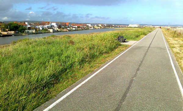
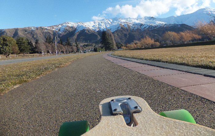
Looking down part of the nice smooth path near the Shoreham Widewater lagoon.
This is a great place to do some basic speed tests, the route being about 1 mile long.
The lagoon is to the left while the sea is on the right.


1 mile data plots

Speed data (mph) v time (seconds from start). The data from about 2000 to 2400 seconds into the journey between the two marker signals (off scale signals) corresponds to a part of the route that was a nice smooth, slightly downhill path (Widewater lagoon). This is good place to get up a steady speed. The speed was obtained simply by multiplying the voltage data by 4.5 (the K value for the IR set-up, see main article above). This part of the trip is about 1 mile long so is very useful for rough calibration. It took 5 mins (300 seconds) to run the mile which therefore an average speed of about 60 / 5 = 12mph. This is close to what we see from the scalled data logger results.

The data between about 2000 and 2400 seconds into the trip is the part from the end of Lancing Green to the start of the road into Shoreham. This is a very smooth, slightly downhill path that is easy to keep a good speed along. The route is so steady that I could crouch down on the board while moving and press the 'marker' button to mark the start of this part of the journey. According to the map this is about 1 mile long. As the journey took 5 mins this corresponds to 1 x 60 / 5 = 12 mph which matches quite well with the scaled data on the plot. You can see from the peaks on this plot that I pushed / skated on the board about 20 times (20 peaks: a push every 15 secs or so) to cover the mile. I then let the board slow down and stopped off for a break and then pressed the marker button to mark the end of this part of the run.


Reds bearings and grease

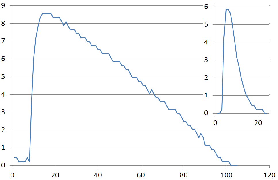
The spin speed (mph equivalent) over time (seconds) of a wheel being spun in air (spinning on its bearing fixed to the truck). The main plot is with new Bones Reds bearings which come with a thin layer of fine oil. The Inset is the same bearings filled with bike grease. The idea of filling with grease is to provide protection from water ingress and also to try and make them less noisy when out and about. Although the grease filled bearings obviously slow down much more quickly when spun in the air, once we are out on the board with our weight (momentum = mass x velocity) this does not slow us down too much. I feel its worth the long term improvement and improved noise reduction.

The data above is the result of adding bike grease to some new bearings. I did this to reduce the noise from the bearings and most importantly to try and minimise water ingress. I found that the new Bones Reds bearings were very good and smooth but were very noisy even on quite a smooth path. The data above shows the way the wheels spin in their bearings when they are simply spun in air (on the truck). For new bearings (which have a very thin layer of fine oil) you can see that wheels spun for 100 seconds or so. When grease is added to the bearings we can see that they do not spin for so long in the air. However once we get on the board our mass (momentum) soon overcomes this friction. Of course you are lossing energy with the thicker grease but the improvement in noise and in keeping water out from the bearings is worth the while.

IR detection
pros: plastic mirror very light weight and cheap. Initial alignment / set-up easy.
cons: may not cope well with very tight bends / steering where the mirror may go out of alignment. Need to keep mirror relatively clean.

Spinning magnet detection
pros: good alignment what ever position trucks take, small component count and lower power than IR set-up.
cons: roads often contain iron 'litter': nails, screws and cleaner brushes, so magnets pick up detritus. Need to be careful about magnet position on different size wheels.


THE CREATIVE SCIENCE CENTRE


Dr Jonathan Hare University of Sussex, Brighton.
e-mail: j.p.hare@sussex.ac.uk

home | diary | whats on | CSC summary | latest news